
Guides & videos
Analysis — the statistical diagnostic of your plots
In a nutshell: Analysis records nothing. It gathers the Plots recorded on one or more parcels of a domain, over a period, and turns them into a statistical diagnostic: the mean value per hectare of each variable, how much it varies from one plot to the next, and the precision of your estimate. The whole thing exports as a Word report, for you to complete.
It is the stand diagnostic tool: it answers the question "what is the growing stock of this parcel?", but also "are my plots enough to say so?".
1. What Analysis computes
The unit of calculation is the plot: a Plot recorded during an observation (see Plot). A single observation can carry several Plots: each one counts as a plot. For each of them, the app already knows the basal area of the different compartments, the density, the regeneration and the deadwood.
Analysis lines these plot values up, variable by variable, and computes their statistics.
The first report available is the Stand condition diagnostic.
2. Choosing the scope
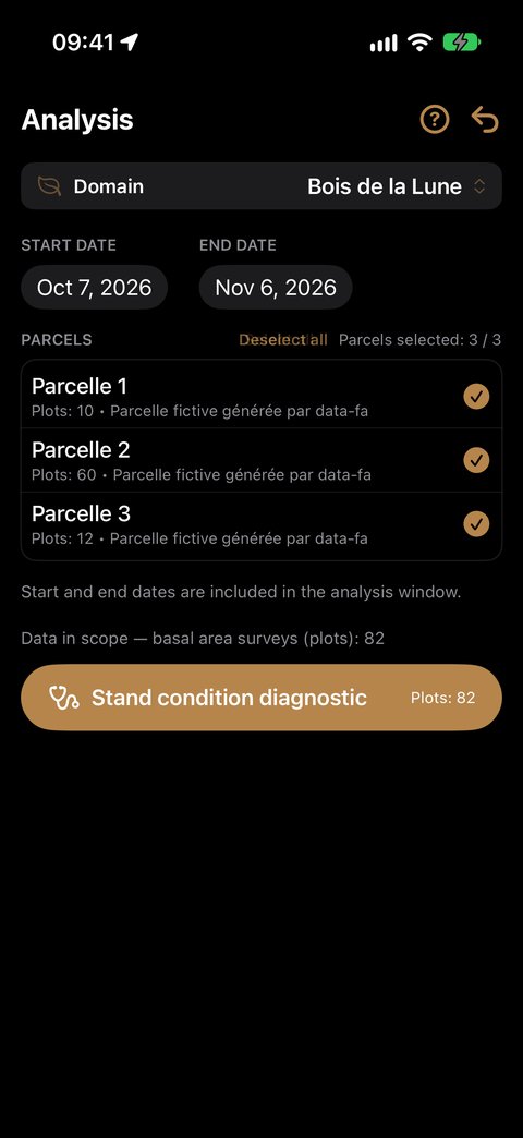
Open Analysis from the home screen. Below the banner, the screen reads from top to bottom.
- Domain: it is the one in the banner, at the top of the screen. To analyse another domain, change it in the banner: the list of parcels follows.
- Start date and End date: the last 30 days are suggested. Both dates are included — a Plot made on the end date counts.
- Parcels: only the parcels carrying at least one Plot during the period appear, each with its number of plots ("Plots: 6"). None is ticked at first: tap those to analyse, or Select all (then Deselect all to start again from scratch). The counter "Parcels selected: 2 / 5" sums it up.
If you change the period, the list follows: a parcel that no longer has a Plot in the new period leaves the list and is unticked; the others keep their state.
Below the list, the app shows how many plots the scope contains. Tap Stand condition diagnostic to run the report; the button stays greyed out as long as no parcel is ticked.
3. The Diagnostic
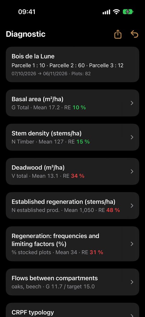
At the top, a reminder of the scope: the domain, each parcel with its number of plots, the period and the total. At the top right, ⇪ creates the Word report (§ 11) and the ↩ arrow takes you back to choosing the scope.
Then come the sections, always in this order:
- Basal area (m²/ha);
- Stem density (stems/ha);
- Deadwood (m³/ha);
- Established regeneration (stems/ha) and Regeneration: frequencies and limiting factors (%), only if at least one plot carries the Regen gesture;
- Flows between compartments, as soon as a plot has living timber;
- Species.
Sections to expand
All sections are closed on opening. Their header already gives the essentials: the key variable, its mean and its relative error, coloured (§ 10). Tap the header to expand the section, tap it again to collapse it.
| Section | Collapsed header |
|---|---|
| Basal area | G Total · Mean · RE |
| Stem density | N Timber · Mean · RE |
| Deadwood | V total · Mean · RE |
| Established regeneration | N established target · Mean · RE |
| Regeneration: frequencies… | % stocked plots · Mean · RE |
| Flows between compartments | the production species, their G and the target G |
| Species | the most represented species, its G timber, its share and its status — for example "oak · G timber 14.2 · 63 % · Objective" |
An expanded section begins with the Definition of its variable: expanded the first time you open the Diagnostic, then collapsed — tap Definition to read it again.
Reading a table
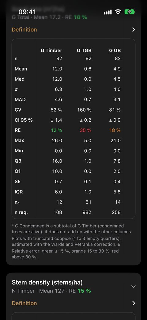
- In columns, the variables: G Timber, G TGB, G GB…;
- in rows, the statistics: n, Mean, Med… (detailed in § 9).
The first column stays fixed; swipe the table to the left to see the other variables. Long-press a statistic's name to show its definition.
A — marks a value that makes no sense for the sample: a standard deviation with a single plot, a coefficient of variation when the mean is zero. A column without any plot is not shown.
4. Basal area, density, deadwood
Basal area (m²/ha)
| Column | What it holds |
|---|---|
| G Timber | the living stems counted with the relascope (Timber gesture), all classes, unclassified included |
| G TGB, G GB, G BM, G PB | the same, by diameter class |
| G Coppice | coppice, estimated with the point-centred quarter method |
| G Pole | the poles in the 10 m circle |
| G Dead | trees standing dead, counted with the relascope |
| G Total | the total basal area: living timber, coppice, poles and standing dead |
| G Condemned* | condemned trees — a subtotal of G Timber |
Stem density (stems/ha)
The same columns, as stems per hectare: N Timber, N TGB, N GB, N BM, N PB, N Coppice, N Pole, N Dead.
A stem counted with the relascope without a diameter class counts in the basal area, but not in the density: its diameter is needed to convert it into stems per hectare. Their number is shown under the table.
Deadwood (m³/ha)
| Column | What it holds |
|---|---|
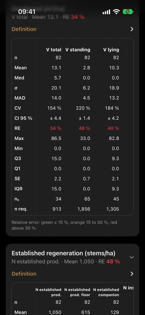
| V total | standing and lying deadwood together, on the plots where the transects were walked |
| V standing | the volume of standing dead trees (11 × G Dead) |
| V lying | the volume of the pieces crossed along the three transects |
5. Zero or "not surveyed": a difference that matters
A plot where a population was surveyed and found absent counts as zero: it is information, and leaving it out would inflate the mean. A plot where it was not surveyed is simply left out of that column. That is why n can change from one column to the next.
| Population | Counts as zero if… | Left out if… |
|---|---|---|
| Timber | no stem counted | — (the relascope sweep is assumed at every plot) |
| Poles | you pressed No poles | no pole and no "No poles" |
| Coppice | all four quarters are empty | no coppice surveyed |
| Lying deadwood | the transects are recorded empty | no transect walked |
| Regeneration | the circles are No seedlings | no Regen gesture, or all circles non-significant |
Plots with truncated coppice (1 to 3 empty quarters) are counted, with an estimate corrected by the Warde and Petranka method: an empty quarter lowers the estimated density. Their number is shown under the table. A shoot of unknown diameter counts as D10, a shoot without a distance counts at 7.5 m.
6. Regeneration
The two Regeneration sections read the circles of the Regen gesture of the Plot. Each plot gives one value, the mean of its retained circles; the statistics then bear on the plots, as for G and N.
Only objective species qualify the regeneration, and for it only production reasons make a species objective: holly, rowan or limes, objective on biodiversity grounds alone, go with the accompanying species.
Established regeneration (stems/ha)
| Column | What it holds |
|---|---|
| N established target | the established seedlings (H2 + H3) of the objective species |
| N established target floor | the same, computed on the minimum counts of the classes: it cannot overestimate, and it is the one compared with the benchmark of 250 stems/ha |
| N established companion | the established regeneration of the accompanying species, for information |
| N installed target | the H1 class of the objective species: what will come next |
Under the table, the Composition of established regeneration (H2 + H3) gives the established density by species, in Objective, Accompanying and No status blocks.
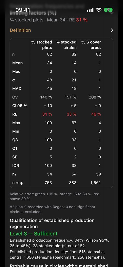
Regeneration: frequencies and limiting factors (%)
| Column | What it holds |
|---|---|
| % stocked plots | 100 if a circle carries established objective regeneration, 0 otherwise: the mean is the frequency, the indicator that matters most |
| % stocked circles, % S cover target | the finer distribution, and the presence of small seedlings |
| % IC, % NC 3 | the share of circles where competition hinders (NC ≥ 2), or blocks (NC = 3) |
| % IG, % NG 2 | the share of circles where the objective species are browsed, or browsed above 50 % |
| % IFL | the share of circles blocked by competition or heavily browsed |
Under the table:
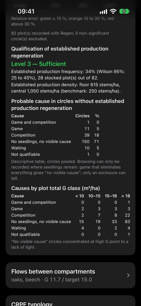
- the Qualification of established target regeneration, in four levels — Absent, Insufficient, Established, Sufficient —, from the frequency (with its Wilson interval) and the floor density;
- the Probable cause in circles without established target regeneration: Game and competition, Game, Competition, No seedlings, no visible cause, Waiting, Not qualifiable;
- the Causes by plot total G class: "no visible cause" circles concentrated at high G point to a lack of light.
7. Flows between compartments
This section draws, in a single diagram, all the compartments of the forest and the flows that link them: the Coppice doses the light at ground level; the Installed regen (S and H1 seedlings) passes 1.5 m to become Established regen (H2, H3), held back by game and competition; the established regeneration passes 7.5 cm and joins the Poles, which recruit the PB, then BM, GB, TGB, from which the Indicative harvest leaves; the Dead wood returns to the soil and prepares the germination beds.
Only production species are counted in it: regeneration made only of hornbeam is worth zero there. Coppice and deadwood remain counted over all their species — the first for its canopy cover, the second because it does not go to harvest.
Each box carries its value and its benchmark: coppice G ≤ 3 m²/ha, poles G from 1 to 3 m²/ha, deadwood V ≥ 30 m³/ha.
| Colour | Meaning |
|---|---|
| green | within benchmark |
| orange | to watch closely |
| red | outside benchmark |
| dotted grey | not recorded, or not qualified |
The timber flow and the target G
The timber frame carries the G of production timber and its target G. The latter combines all the production species of the parcel: the equilibrium range of each genus (oaks 14-19, beech 15-22, chestnut 15-25, pines 20-30, Douglas fir and firs 25-40 m²/ha) is weighted by its share of G, and the target G is the middle of the resulting range. Oaks 70 % and beech 30 % thus give 14.3-19.9, target 17.1. A production species with no known range (ash, wild cherry, maple…) does not enter this calculation.
Above the frame, the diagram recalls the distribution of the production species and the GB + TGB rule, whose target is half of G. Under the PB to TGB boxes, a grey band gives the G of the condemned trees, included in the timber G.
The Indicative harvest box shows the gap between the timber G and the target G when it exceeds it; otherwise, it reads "Capitalising: no harvest". It is not a recorded felling: the app does not record fellings.
Enlarging the diagram
Tap the diagram, or its magnifier, to open it full screen. Pinch to enlarge it (up to five times), drag it with your finger, double-tap to enlarge or return to scale. The ↩ arrow takes you back to the Diagnostic.
8. Species
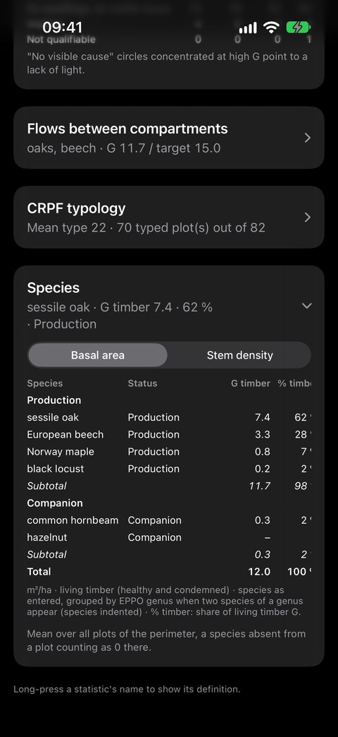
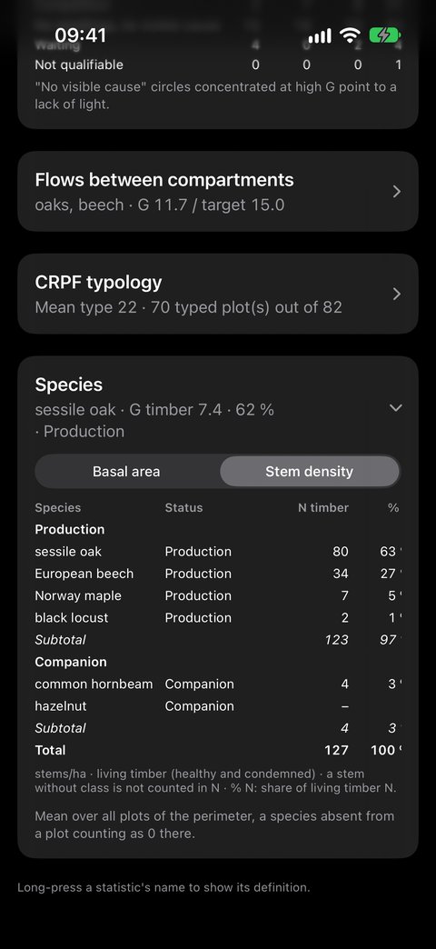
The last section breaks the living timber down by species, over the whole scope: each value is the mean over all plots, a species absent from a plot counting as zero there. The species are those you entered; two species of the same genus are grouped under the genus row, the species indented.
Two tabs at the top of the table:
- Basal area: G timber, % timber, G TGB, G GB, G BM, G PB, G coppice, G pole, in m²/ha;
- Stem density: N timber, % N, N TGB, N GB, N BM, N PB, N coppice, N pole, in stems/ha.
The Status column, just after the species, shows Objective, Accompanying or To be documented; "–" for a species not entered or unknown. The table is split into Objective, Accompanying, then No status blocks where applicable, each with its Subtotal; the Total row closes the table. Within each block, species are ranked from most to least represented.
9. The statistics, row by row
| Row | Name | What it tells you |
|---|---|---|
| n | Count | the number of plots used for the column |
| Mean | Mean | the estimate of the variable per hectare for the scope |
| Med | Median | half the plots above, half below; a large gap with the mean betrays a few extreme plots |
| σ | Standard deviation | the spread around the mean: about two plots in three lie within one standard deviation |
| MAD | Mean absolute deviation | the average distance from a plot to the mean, less sensitive to extremes |
| CV | Coefficient of variation | the standard deviation relative to the mean, in %: the higher it is, the more heterogeneous the stand |
| CI 95 % | 95 % confidence interval | the true mean has 95 chances in 100 of lying within Mean ± CI |
| RE | 95 % relative error | the CI relative to the mean, in %: the precision of your estimate |
| Max · Min | Extreme values | the highest and the lowest plot |
| Q3 · Q1 | Quartiles | three quarters / one quarter of the plots below this value; half the plots lie in between |
| SE | Standard error of the mean | the uncertainty on the mean itself (σ / √n) |
| IQR | Interquartile range | Q3 − Q1: the range of the middle half of the plots |
| n₀ | Zero plots | how many plots have none of this population |
| n req. | Required plots | how many plots would be needed for a 10 % relative error |
10. Precision: should you add plots?
The RE row, like the header of each section, is coloured:
| Colour | Relative error | Reading |
|---|---|---|
| Green | up to 15 % | a solid estimate |
| Orange | 15 to 30 % | to be consolidated |
| Red | above 30 % | too imprecise to decide on |
The relative error falls as plots are added, but slowly: it takes four times as many plots to halve it. The n req. row does the maths for you — if it reads 19 and you have 12, seven more plots would bring the error down to 10 %.
11. The Word report
The Diagnostic is read on screen; the report puts it into a Word document (.docx) that you complete as you wish — comments, photos, conclusions — before including it in a field report, a marking or a management plan. It opens in Word, Pages, LibreOffice or Google Docs, on a computer as on the iPhone.
Creating the report
- Choose the scope (§ 2) and open the Diagnostic.
- Tap ⇪ at the top right, next to the back arrow.
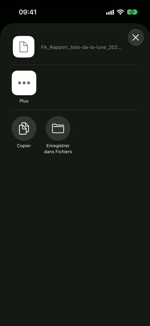
- The share sheet opens: save the document in Files, send it by Mail or AirDrop, or open it directly in Word or Pages.
The report covers the scope shown — the domain, the ticked parcels and the period. It is written in the language of the app.
What it contains
| Part | Content |
|---|---|
| Header | the name of the domain, the period, the selected parcels, the creation date and the app version |
| Domain summary | municipality, reference point, manager and forester, number and area of the parcels, share of the area covered by the report, domain map, activity during the period (observations and surveys), table of the parcels of the domain with their number of plots |
| Summary by parcel | one table per section, with one row per parcel and an All row: means, count, coloured relative error. This is the page that compares your parcels |
| Whole scope | the on-screen Diagnostic, all plots pooled, and its flow diagram |
| One part per parcel | the parcel map, its own diagnostic, its flow diagram, then its breakdown by species |
| Appendix | the method, the definition of each variable and each statistic |
The footer of each page recalls the title, the app version and the page number. The sections follow the order of the screen; they are all expanded there.
The breakdown by species of each parcel
Each parcel part ends with its Breakdown by species: the table of the Species section, computed on the plots of the parcel, in basal area then in density, with the Status column and the Objective, Accompanying and No status blocks. This is where you read the composition specific to each parcel, which the screen, pooling the whole scope, does not show.
The domain map
It shows all the parcels of the domain: those that are part of the report are in green, with their name in bold; the others remain in grey. The black dots are the plots of the period. A legend, the scale and the north arrow accompany the map.
The map of each parcel: the timber distribution
At the top of a parcel's part, its map places each plot at its position. Each plot is a pie chart showing the timber distribution:
| Colour | Class |
|---|---|
| yellow | PB — small timber |
| orange | BM — medium timber |
| dark orange | GB — large timber |
| brown | TGB — very large timber |
Each slice is the share of the class in the basal area of the plot's living stems: an almost brown pie chart flags a plot capitalised in large timber, a yellow pie chart a young plot. An empty circle is a plot with no classified stem. Stems counted without a diameter class do not enter the pie chart.
The maps are drawn from your parcels and your Plots, without a base map: the report is obtained offline, in the forest as in the office.
12. In short
- Plots made in the right parcels;
- No poles and Empty transect so that zeros count;
- the domain is chosen in the banner, the parcels are ticked by hand;
- one scope = one sample: the Word report compares the parcels;
- expand the sections; look at n, then Mean, then the colour of RE;
- n req. tells you how many plots to add;
- ⇪ in the Diagnostic: the Word report, to complete, with the maps and the breakdown by species of each parcel.
What next
- Recording a Plot — the gestures that feed the Diagnostic, including Regen
- Exporting your data — to work on your surveys outside the app